
Performance metrics for binary Classification models
A deep dive into performance metrics for Machine learning models for classification models and selecting the best metric based on business scenario
Metrices play an important role in determining the performance of a machine learning model. Even more important use case of metrices is to benchmark and report the performance across board.
There is a large set of metrics available to chose from, but pertaining to one’s business problem, it becomes critical to select the right metric that can do justice to the business use case that we are trying to solve. Interpreting these metrices in layman’s term is also very important as often we need to explain the performance in terms of these metrices to end users who are not ML Scientists or Data Scientists. Without further due, let us jump into different metrics, their definition, and best suited use cases.
List of metrics we will cover in this section:
- Confusion matrix
- Accuracy score
- Precision score
- Recall score
- F1 score
- F-beta score
- Area under curve (AUC) & Receiver Operating Characteristic (ROC)
Confusion matrix
Confusion matrix, as the name suggest, measure how confusion the model is in predicting the classes. Let us consider the following table to understand how the confusion matrix is actually used:

Confusion matrix is the fundamental to most of the metrics that we will discuss in this post. As we move forward, we will see how every metrics (except AUC-ROC) can be easily determined from the confusion matrix. So it is important that we understand the confusion matrix thoroughly.
Code snippet for python:
from sklearn.metrics import confusion_matrix
# if you want frequency
confusion_matrix(y_true, y_predicted)# if you want the normalized frequency distribution
confusion_matrix(y_true, y_predicted, normalize='true')
A confusion matrix, as seen from the image above, is a cross tabulation of the Actual (True) classes (represented as rows) and Predicted classes (represented as columns). For binary classification case, where 0 represents negative event and 1 represents positive event, we will have 4 cells corresponding to each of the combination: {Actual, Predicted} as below:
{0, 0} = True Negative: when true class is 0 and model also predicted it as 0,
{1, 0} = False Negative: when true class is 1 but model predicted as 0,
{0, 1} = False Positive: when true class is 0 but model predicted as 1
{1, 1} = True Positive: when true class is 1 and model also predicted as 1
Clearly from the above, having higher TP and TN with minimum FP and FN is the desired state. But in practice, it works bit differently — not all 4 cells can be optimized (maximized or minimized) at the same time. For example, when we try to maximize TP, FP also starts increasing and similarly, when TN increases, FN also increases. Now the bigger question here is how should we determine what will be the optimum value or the best selection for a model. This is where other metrices developed based on the confusion matrix plays an important role.
Accuracy score
This is the most commonly used scored in any classification problem. Accuracy score measures how accurately the model predicts the classes — out of total population, how many of the 0’s are correctly predicted as 0 and how many of the 1’s are correctly predicted as 1. Using the confusion matrix, it can be represented as:

Code snippet for python:
from sklearn.metrics import accuracy_score

accuracy_score(y_true, y_predicted)
While accuracy score is a good representative of the model performance in case of equally distributed classes, it suffers from drawbacks like — in case of an skewed data where we have 99.99% 0’s and only 0.01% 1’s, accuracy score does not make much sense. If the model predict every record as 0, the accuracy score will still be 99.99%. To overcome this problem, let us look into other metrices which help us to assess the performance of model and align it with business objective.
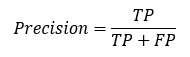
Precision score
Precision helps us estimate the percentage of cases which are actually (true class) 1’s out of the total predicted 1’s. Using the confusion matrix, precision can be computed as:
Code snippet for python:
from sklearn.metrics import precision_score

precision_score(y_true, y_predicted)
Measuring precision becomes very important when misclassifying an example as positive when it is not actually positive is costly. For example, in prediction of attrition where existing customers are offered a heavy discount will be very costly if precision is low, i.e. customers who are less likely to attrite will be provided with heavy discount leading to huge business loss.
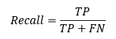
Recall score
Recall helps us estimate the percentage of cases which are predicted as 1’s out of total cases where the actual class is 1. Using the confusion matrix, precision can be computed as:
Code snippet for python:
from sklearn.metrics import recall_scorerecall_score(y_true, y_predicted)
Recall is the go to metric in cases where failure to detected a positive case is very costly. For example, in a marketing campaign, every failure to detect a customer who is likely to buy the product will be a loss of opportunity.
F1 score
There are cases, where maintaining a balance between precision and recall is of importance rather than looking at any one of these metric in standalone. This is where F1 score plays an important role. F1 score is the harmonic mean of precision and recall. Mathematically, F1 score is computed as:
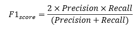
The usage of harmonic mean in computing F1 score makes the score robust and reduces the impact of extreme cases.
Code snippet for python:
from sklearn.metrics import f1_scoreprecision_score(y_true, y_predicted)
F1-score becomes important in cases, where both precision and recall are equally important and balance needs to be made between these two scores. But how about the cases where different weightage needs to be put for precision and recall? To address this problem, F-beta score is designed where importance on one metric (Recall) can be specified. Let us look into it in the next section.
F-beta score
F-beta score is the weighted version of F1 score. F-beta introduces a new hyper-parameter β, which is chosen in a way that recall is considered β times as important as precision. Mathematically, F-beta score is computed as:
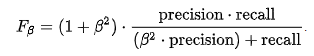
When β= 1, F-beta is same as F1 score as precision and recall becomes equally important. When β < 1, more weightage is put on precision and when β > 1 more weightage is put for recall.
Code snippet for python:
from sklearn.metrics import febta_scorefebta_score(y_true, y_predicted, beta=0.5)
F-beta score becomes very useful in use cases where more weightage needs to be put on recall maintaining the precision or in cases where the focus needs to be more on precision at the same time recall being maintained.
AUC-ROC score
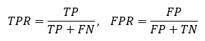
AUC or Area under the ROC curve is simply the probability that an example from positive class (1) will have higher score generated by the model as opposed to an example from the negative class (0). ROC or Receiver operating characteristic chart is built by plotting Sensitivity (or True Positive Rate: TPR) on the y-axis and (1 — Specificity) (or False Positive Rate: FPR) on the x-axis.
Code snippet for python:
from sklearn.metrics import roc_curve, auc# first false postive rate (fpr) and true positive rate (tpr) need
# to be extracted using roc_curve function
fpr, tpr, thresholds = roc_curve(y_true, pred_probability)# pass the computed fpr and tpr into auc function to get score
auc(fpr, tpr)
AUC score is most commonly used in highly unbalanced data — where the number of positive cases (1) is much much lower than the number of negative (0) cases.
Conclusion
In the above sections we have seen few key metrices that are commonly used in measuring the performance of a classification model. However, the choices of these metrics depends on the business use case and the problem that is intended to solve. While confusion matrix is the common one across models, other metrices depends on the cost impact of misclassification of labels and how is data (dependent variable) is distributed.
That will be all about metrices and their usage in the context of binary classification. Hope it was helpful.
If you like it, do follow me for more such posts ☺.
